All published articles of this journal are available on ScienceDirect.

Comparative Analysis of Hyperparameter Optimization Techniques for PCA–XGBoost Models in SRCFSST Column Load Prediction
Abstract
Introduction
This study aims to predict the peak axial load capacity (PALC) of steel-reinforced concrete-filled square steel tubular (SRCFSST) columns under elevated temperatures using a machine learning-based approach. The motivation arises from the limitations of traditional experimental and numerical methods, which are often time-consuming, costly, and computationally intensive.
Methods
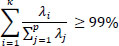
A hybrid predictive framework was developed by integrating Principal Component Analysis (PCA) with Extreme Gradient Boosting (XGB). The dataset, comprising 135 instances from prior experimental studies, underwent PCA for dimensionality reduction, retaining 99% of the variance. The PCA-transformed data was used to train XGB models, with hyperparameter tuning conducted via Grid Search, Random Search, and Bayesian Optimization. A 5-fold cross-validation technique was employed to enhance model generalizability, and performance was evaluated using R2, RMSE, and WMAPE.
Results
Among the three tuning strategies, the Bayesian-optimized PCA-XGB model demonstrated the highest predictive performance with an R2 of 0.928, MAE of 2.3%, and RMSE of 3.5% on the test dataset. Statistical analyses, including paired t-tests and Wilcoxon signed-rank tests, confirmed the superiority of this model with significant improvements over other configurations (p < 0.05). The use of PCA notably reduced multicollinearity and computational complexity.
Discussion
The findings underscore the value of combining dimensionality reduction with advanced hyperparameter tuning to develop efficient, accurate, and interpretable models for structural fire engineering. The PCA-XGB-BO framework offers a viable alternative to traditional modeling approaches, particularly for complex prediction problems involving high-temperature effects on structural components.
Conclusion
This study establishes a robust data-driven methodology for estimating PALC in SRCFSST columns exposed to high temperatures. The integration of PCA and Bayesian Optimization within an XGB modeling framework delivers high accuracy while reducing computational burden. Future research should focus on extending this framework to other structural systems, incorporating physics-informed constraints, and validating performance through large-scale experimental testing.
1. INTRODUCTION
Concrete-filled steel tubular (CFST) columns are gaining traction as essential components in building construction because of their high strength-to-weight ratio, effective construction techniques, and ability to withstand earthquake forces [1]. The parts formed from these materials can efficiently provide structural support to tall structures, bridges, and numerous other load-bearing structures owing to the tensile and ductile qualities of steel while utilizing the compressive strength of concrete [2, 3]. The shape and structural geometry of CFST columns eliminate the disadvantages of space and weight for extremely tall buildings because they have a low volume to resist lateral forces [4, 5]. Despite these advantages, CFST columns' performance under extreme scenarios, particularly prolonged exposure to high temperatures during fire events, remains a critical concern. These columns are particularly effective in buildings exposed to prolonged fire conditions, as the concrete inner core acts as an insulator, protecting the steel by slowing down heat transfer [6]. However, it is essential to understand how CFST columns respond to extreme heat to maintain structural stability in irresponsible situations such as fire outbreaks. There is a great risk that the high temperature may damage both the steel tube and concrete core, which raises concerns regarding the structural properties of the CFST columns and, consequently, the safety of the building system [7, 8].
Some experimental research has been carried out to assess the thermal and mechanical properties of CFST columns exposed to high temperatures. Franssen and Kodur (2001) conducted fire tests to analyze the fire resistance of such columns, observing the dominant effect of temperature on the load-carrying capacity of structures [9]. Similarly, the fire behavior of CFST columns has been investigated in terms of their residual strength, with studies concluding that a certain portion of the load-bearing capacity can be retained after cooling, owing to the thermal choking effect of the concrete core [10]. Nevertheless, despite the valuable insights gained from these experimental studies, their practical applicability is limited by factors such as high costs, preparation complexity, standardized testing conditions, and the unpredictable nature of real-world scenarios. On top of that, the high variety of concrete mixtures and steel types utilized in CFST columns renders a conclusion drawn from the experiments less convincing.
While experimental investigations yield useful information, practical considerations like cost, controlled environments, and variations in material composition point to the necessity of looking beyond. Numerical methods have, therefore, been utilized to model the performance of CFST columns during fire exposure. The finite element modeling (FEM) method was utilized to calculate the thermal profile and thermal stresses within the CFST columns following exposure to fire. These researches have shown accurate predictions of CFST structural behavior, such as but not restricted to thermal gradients, on the individual elements of CFST and the geometry of the whole column [11, 12]. Finite element models are beneficial for researchers who want to investigate the effects of specific parameters without having to perform physical tests [13]. However, such methods are time-consuming and need extensive material property information in order to find the correct results [14].
Recent research has extensively studied the structural performance of steel–concrete composite systems. Song et al. highlighted the significant impact of flange thickness and foundation stiffness on the shear contribution via dowel action in steel–concrete–steel composite structures [15]. Researchers reported improved ductility and energy dissipation in rubberized concrete-filled steel tubes despite reduced concrete strength [16, 17]. Nie et al. confirmed that uplift-restricted and slip-permitted screw-type connectors significantly enhance crack resistance and seismic resilience in composite frames without considerably affecting structural bearing capacity [18].
Owing to the limitations in performing numerical simulations of fire scenarios, such as modeling of nonlinear thermal and mechanical responses, other methods have been explored by scientists. Given the challenges associated with both experimental and numerical approaches, there has been a growing interest in data-driven modeling techniques, particularly soft computing and machine learning, for evaluating the performance of CFST columns under extreme conditions.
Soft computing techniques have undergone significant advancements over the past few decades, initially finding widespread applications in medical and healthcare domains before being increasingly adopted in engineering disciplines. Early implementations primarily focused on solving complex biological and epidemiological challenges, such as modeling pandemic risks, genetic susceptibility in severe diseases, and AI-driven predictive diagnostics [19-21]. These approaches leveraged heuristic algorithms, artificial neural networks (ANNs), and machine learning frameworks to enhance medical decision-making and disease prognosis. Over time, the success of soft computing in medical applications catalyzed its integration into engineering fields, where challenges such as high-dimensional data, uncertainty, and nonlinearity necessitate more advanced computational techniques. In structural and geotechnical engineering, data-driven approaches incorporating soft computing have revolutionized predictive modeling, optimization, and reliability assessment. Recent advances in artificial intelligence and hybrid learning models have enabled precise estimations of material behavior, structural stability, and fire resistance in critical infrastructure. The integration of machine learning with hyperparameter tuning techniques, as demonstrated in this study, exemplifies how soft computing principles have evolved from medical diagnostics to engineering solutions, bridging computational intelligence with real-world structural challenges [21].
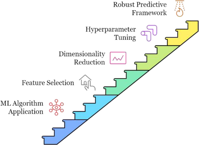
The work done by Researchers has demonstrated that various machine learning frameworks, such as artificial neural networks (ANN) and support vector machines (SVM), can be reliably used to estimate the axial capacity of concrete-filled steel tubular (CFST) columns [22, 23]. All ML models were fitted to experimental and simulated data to learn the axial load capacity as a function of several input variables, including the material properties and column dimensions. Although they have proven to be good at making these predictions, such methods tend to ignore the possibility of using these approaches for feature selection and data dimension reduction, which improves the efficiency of the model and the clarity of its interpretation [24, 25]. Despite the positive outlook on ML solutions for design problems, several issues still require further research. Several studies have applied regular machine-learning algorithms in the absence of any attempts to redesign the feature space, which often causes overfitting and a lack of generalizability to other datasets [26]. The contribution of dimensionality reduction techniques, such as Principal Component Analysis (PCA), has not been adequately discussed in this field, despite their ability to reduce the complexity of the input data and enhance the computational speed without losing the prediction capability. Moreover, hyperparameter tuning, which is a crucial strategy for the improvement of machine learning models, particularly with SRCFSST column systems (Fig. 1), has not been addressed. Research comparing approaches such as grid search, random search, and Bayesian search with respect to their effectiveness in tuning models that forecast the behavior of SRCFSST at elevated temperatures is also scarce.
This research is motivated by the hypothesis that the combination of Principal Component Analysis (PCA) with Extreme Gradient Boosting (XGB) and optimized hyperparameter tuning methods greatly improves the predictive precision and efficiency of peak axial load capacity (PALC) prediction for high-temperature steel-reinforced concrete-filled square steel tubular (SRCFSST) columns. In order to test this hypothesis, the research aims to answer three major research questions. First, it explores the efficiency of the PCA-XGB model in the prediction of the PALC of SRCFSST columns in comparison with conventional experimental and numerical methods. Second, it analyzes the relative performances of various hyperparameter search methods—Grid Search (GS), Random Search (RS), and Bayesian Optimization (BO) —with the aim of identifying their contribution to enhancing model accuracy and resilience. Third, it investigates whether the incorporation of dimensionality reduction methods like PCA can reduce overfitting risks and improve the computational efficiency of machine learning-based predictive models for structural fire engineering applications.
By addressing these research questions, this study aims to fill existing gaps in the application of machine learning for structural performance prediction under fire conditions. The suggested methodology (Fig. 2) consists of analyzing the PALC of SRCFSST columns at high temperatures. To do this, we employed XGB and PCA-enhanced XGB. This research effectively utilizes PCA due to its ability to reduce the dimensions of the data, which simplifies the data and is expected to improve the model's robustness. Besides, various hyperparameter tuning methods, including grid search, random search, and Bayesian Optimization, have also been examined in order to improve the performance of the model in accuracy as well as efficiency.
This research stands out for its comprehensive approach, as it combines PCA and advanced hyperparameter tuning with XGB to develop a robust predictive system for SRCFSST columns exposed to high temperatures. By explicitly formulating the hypothesis and research questions, this study provides a structured framework that enhances the reader’s understanding of the research objectives, methodology, and contributions to the field of structural fire engineering. The findings not only contribute to the advancement of machine learning applications in fire-resistant design but also lay the foundation for future studies exploring intelligent computational methods for predicting structural element failure under extreme loads.
2. METHODOLOGY
The methodology shown in Fig. (3) employed to forecast the PALC of SRCFSST columns at elevated temperatures involves integrating PCA for dimensionality reduction with XGB for predictive modeling. The dataset containing 135 data points was first standardized to ensure uniform contribution from all features. In order to optimize the performance and effectiveness of the machine learning models, Linear Normalization was employed to standardize the raw data. This technique, as described [27], scales all independent variables to a range between 0 and 1, utilizing the equation provided [27].

Cross section of SRCFSST column.
Progressive steps in model development and evaluation framework.
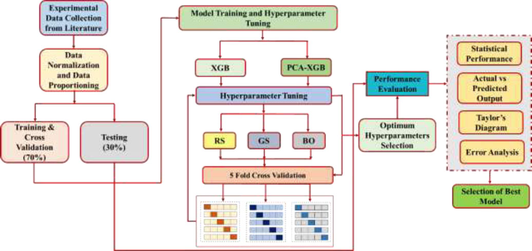
Methodology flowchart.
A covariance matrix was computed to examine interdependencies among input parameters, and eigenvalues and eigenvectors were derived, allowing the identification of principal components that best capture data variance. The selection of principal components was based on 99% cumulative variance, reducing the feature set while retaining essential information. The transformed dataset, now with reduced dimensions, was utilized as the input for the XGB model.
After normalizing the dataset, 70% was used for training and the remaining 30% was used for testing. The training set was also used for cross-validation purposes and to adjust the hyperparameters of the XGB model. To increase the reliability of the predictions, a 5-fold cross-validation method was used during the training course. To improve model performance, three hyperparameter optimization techniques, grid search, random search, and Bayesian optimization, were employed.
PCA was used to address issues of high dimensionality and potential multicollinearity in the input data, both of which could have adverse effects on model correctness. This technique reduced the dataset and increased the prediction accuracy by reducing the input variables to five main components, which captured 99% of the cumulative variance while retaining crucial information from the original dataset. The resulting condensed dataset was utilized to build a new PCA-XGB model.
The tuning and cross-validation of the PCA-XGB model were performed in the same way as those of the original XGB model, with hyperparameters fine-tuned using grid search, random search, and Bayesian optimization. The specific ranges of hyperparameters tested during each tuning technique were carefully selected to ensure a comprehensive optimization process. Grid Search (GS) systematically evaluates a predefined range of hyperparameter values by testing different configurations, including the number of boosting rounds (n_estimators) set at 100, 200, 300, and 400, the learning rate (learning_rate) varied at 0.01, 0.05, 0.1, and 0.2, the maximum depth of trees (max_depth) explored at 3, 5, 7, and 9, the subsample ratio of training instances (subsample) considered at 0.6, 0.7, 0.8, and 0.9, and the column sample ratio (colsample_bytree) tested at 0.3, 0.5, 0.7, and 0.9. Random Search (RS) takes a different approach by selecting hyperparameter combinations randomly from a broader search space to explore diverse values with a reduced computational cost. The tested ranges for Random Search included the number of boosting rounds (n_estimators) between 100 and 400, the learning rate (learning_rate) varying from 0.01 to 0.2, the maximum depth of trees (max_depth) between 3 and 9, the subsample ratio of training instances (subsample) ranging from 0.5 to 0.9, and the column sample ratio (colsample_bytree) set between 0.2 and 0.8. In contrast, Bayesian Optimization (BO) employs a probabilistic model to dynamically refine the search space, ensuring a more efficient search for optimal hyperparameter configurations. The hyperparameter search space for Bayesian Optimization included the number of boosting rounds (n_estimators) ranging from 150 to 400, the learning rate (learning_rate) between 0.01 and 0.15, the maximum depth of trees (max_depth) varying from 4 to 10, the subsample ratio of training instances (subsample) between 0.6 and 0.9, and the column sample ratio (colsample_bytree) within the range of 0.3 to 0.9. Bayesian Optimization provided the best hyperparameter combination, achieving superior performance with the lowest Root Mean Square Error (RMSE) and highest R2 score. The optimized PCA-XGB model was tested on 30% of the dataset, confirming its predictive accuracy in estimating SRCFSST column axial load capacity under high-temperature conditions. The enhanced implementation details of PCA and XGB now ensure full transparency, facilitating the replication of this study by researchers and practitioners.
This detailed explanation of the hyperparameter search space ensures transparency regarding the scope of optimization and the computational considerations involved in the tuning process, providing clarity on how each optimization technique was implemented to enhance the predictive performance of the PCA-XGB model. The selection of hyperparameters was based on their impact on model generalizability and prediction accuracy, ensuring that the final tuned models achieved optimal performance.
After determining the best parameters, the XGB and PCA-XGB models were tested on a 30% sample of the data to assess their precision in forecasting the PALC of the SRCFSST columns under elevated-temperature conditions. This extensive approach enabled a rigorous assessment of the model's correctness and efficiency, resulting in a robust methodology for forecasting the PALC of SRCFSST columns under high-temperature conditions.
3. COMPUTATIONAL METHOD AND PRINCIPAL COMPONENT ANALYSIS
3.1. Extreme Gradient Boosting
Extreme Gradient Boosting (XGB) is a sophisticated machine learning algorithm that enhances predictive accuracy by combining multiple decision tree models within an ensemble framework [28]. It is widely recognized for its performance across diverse application areas and excels in structured data analysis through iterative learning from multiple trees [29]. XGB has since evolved into one of the most reliable and efficient algorithms in the field [30]. Its fundamental goal is to optimize a given loss function using gradient descent techniques, thereby minimizing prediction error during training [27, 31].
In XGB, the objective function consists of two main components: a loss function and a regularization term. The loss function measures the difference between the predicted outcomes and the actual target values, guiding the model toward better accuracy [27]. Unlike traditional Gradient Boosting Machines (GBM), XGB includes a regularization term that helps control model complexity and prevents overfitting, thereby improving the model’s generalization capability [28, 31-33].
XGB follows a level-wise growth strategy in algorithmic tree design, increasing efforts towards tree construction by depth. Although computationally expensive, this approach reduces model performance. The algorithm introduces an objective function for loss aversion and weight penalties to curtail overfitting. It implements a shrinkage factor for each added tree, reducing tree strength and allowing model improvement. XGB builds trees by sampling training sets column-wise, helping to humble the model and minimize overfitting. These factors make XGB a strong predictive modeling technique [34].
3.2. Principal Component Analysis
Hotelling popularized PCA, a widely utilized method in science and engineering research [35]. PCA is a dimension-reduction method that converts a set of correlated attributes into a fewer number of uncorrelated components called principal components. Not only does this reduce the complexity of data interpretation, but it also increases efficiency in computation since the original data set is depicted using fewer variables with the most variance maintained.
The process of transformation in PCA is founded on the eigenvalue decomposition of the covariance matrix, wherein the principal components are chosen in terms of the eigenvalues that they are associated with. They are ordered in the decreasing order of variance, and the first principal component retains the maximum possible variance in the dataset, followed by the next components in the declining order. As such, PCA correctly selects the most important features of a dataset and hence enables enhanced analysis and decision-making. The detailed mathematical representation of PCA appears in a few studies [27, 36].
In practical implementation, PCA follows these key mathematical steps to achieve dimensionality reduction:
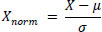
3.2.1. Standardization
To ensure that all features contribute equally, the dataset is standardized by subtracting the mean and dividing by the standard deviation for each feature. Given a dataset X with n observations and p features, the standardized value Xnorm is given by Eq. (1)
 |
(1) |
where μ is the mean and σ is the standard deviation of each feature.
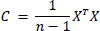
3.2.2. Covariance Matrix Calculation
The covariance matrix C is computed using Eq. (2) to analyze the relationships between features.
 |
(2) |
This matrix captures the variance within each feature and the covariance between different features.
3.2.3. Eigenvalue Decomposition
PCA transforms the dataset by identifying eigenvalues and eigenvectors of the covariance matrix as given in Eq. (3)
 |
(3) |
where λ represents the eigenvalues, and v represents the corresponding eigenvectors.
3.2.4. Principal Component Selection
The eigenvectors corresponding to the highest eigenvalues constitute the principal components. These components are arranged in descending order based on their variance contribution, calculated using Eq. (4), and the first K components are selected such that they retain the majority of the variance.
 |
(4) |
In this study, Principal Component Analysis (PCA) was employed to reduce the dimensionality of the dataset from 11 features to five principal components, which retained 99% of the cumulative variance. This selection facilitated the model's focus on the most informative features while eliminating redundant and correlated attributes.
3.2.5. Transformation to New Feature Space
The original dataset X is projected onto the new feature space defined by the selected eigenvectors using Eq. (5)
 |
(5) |
where VK is the matrix of the top K eigenvectors.
By applying PCA, the dataset was transformed into a lower-dimensional space, improving computational efficiency and reducing the risk of overfitting in the machine-learning model. The integration of PCA with XGB ensured that only the most critical information was retained, leading to improved predictive performance.
3.3. Hyperparameter Tuning, Optimization and 5-Fold Cross-validation
It is necessary to select an appropriate optimization approach for hyperparameter tuning for an effective performance configuration. In traditional optimization techniques, the technique is not very effective in hyperparameter tuning because most hyperparameter tuning problems are non-linear or non-smooth optimizations that are more likely to be trapped locally rather than global optima. For instance, methods based on gradient descent are often employed in reinforcement learning to modify hyperparameters that are continuous in nature, such as the learning rates in neural networks [37]. However, unlike popular methods, such as gradient descent, a number of other strategies have emerged that are more relaxed than HPO [38]. For instance, decision-theoretic frameworks, Bayesian optimization, multi-fidelity optimization, and metaheuristic approaches offer more management power and efficacy for both continuous and discrete hyperparameters.
Decisions in decision-theoretic approaches are made by defining a hyperparameter exploration space and searching for the best combinations available within the space. Grid search (GS) and random search (RS) are two of these techniques. GS examines all the hyperparameter values within a specific boundary or range [39]; in contrast, RS takes certain bays of hyperparameter values at random [40]; thus, it is more economical to use resources in, for instance, hyperparameter tuning than GS. Each of these strategies assesses the performance of all the tuning parameter settings separately.
In contrast, unlike GS and RS, Bayesian optimization (BO) avoids wasting evaluation trials by using selectively tested hyperparameter values to inform the next selection [41]. In this way, because the distribution of the objective function is represented using surrogate models such as Gaussian processes (GP), random forests (RF), or the tree-structured parzen estimator (TPE) [42], BO can reach its optima in a small number of iteration cycles. Conditional hyperparameters such as kernel type and penalty parameter C in support vector machines are presented in BO-RF and BO-TPE as extensions. However, as BO works iteratively with the view of going into unexplored territories and making use of already explored spaces, incorporating parallelization is not straightforward [43].
Concerning overfitting, the optimization of hyperparameters is fundamental for achieving better accuracy in XGB models [44]. The outcomes of machine-learning models are highly dependent on the choice of hyperparameters, particularly when the model is desired to perform optimally. In the past, the fine-tuning of hyperparameters was performed through a trial-and-error process, which involved a grid search, whereby a fixed number of specific values for the parameters were tested. This research also focused on the tuning of the XGB model, which is widely applied in practice: grid search, random search, and Bayesian optimization. All methods are different in terms of the hyperparameter space sampling strategy and focus on performance vs. computational resource limits.
The grid search checks all the possible configurations of the selected hyperparameters in a certain hyperparameter space or grid. In the case of XGB, the most important hyperparameters that are tuned are the number of boosting rounds (or trees) and the learning rate. On the contrary, a random search takes any combination of hyperparameters to the specified limits, using less time and effort when there are many parameters to optimize. Probably the most complicated method, Bayesian optimization, also searches for hyperparameters, but it does this based on the results obtained during previous evaluations and uses probabilistic models for this purpose, thus looking for the hypotheses in a more focused manner and doing so usually quicker than by searching all the possibilities.
To enhance the tuning results and minimize bias, 5-fold cross-validation (CV) was adopted. Five equal parts of the dataset were obtained using this approach, four of which were used to train the model and one to validate it. This process was repeated until the last fold was used as a test set. This CV technique provides a better approximation of the effectiveness of the trained model while minimizing the chances of overfitting the model and allows the tuning results to be applicable to new samples. For this reason, a combination of grid search, random search, and Bayesian optimization, along with a 5-fold CV, is used to enable thorough and effective tuning, leading to the best possible XGB model being built.
4. DATA ACQUISITION AND PROCESSING
A total of 135 data entries were compiled from existing experimental research focused on the behavior of SRCFSST columns under elevated temperature conditions. These entries encompass essential structural and material parameters recorded across varying heating durations and thermal exposures [45]. The key input parameters include the square steel tube wall thickness (t) and area (Ast), section steel dimensions (depth (h), flange width (b), web thickness (tw), flange thickness(tf), and area (Ass)), time of exposure to heating (T), among other factors such as concrete properties, compressive strength (fc), and area of concrete (Ac). The output variable was the PALC (Pu).
To avoid inconsistency and scale differences between various features, the dataset was normalized and standardized prior to model training. Min-max normalization (Linear Normalization) was used for scaling all the independent variables between 0 and 1, so that no parameter overpowered the model by being on a larger scale. It serves to preserve relative feature relationships for better learning by tree-based models like XGB, which do not need normally distributed input data.
Besides min-max normalization, z-score standardization was also performed in order to examine feature distributions and identify possible outliers. The technique standardizes data in terms of having zero mean and unit variance, making sure that variations among features are properly scaled. The z-score examination and KDE plot again checked the normalization process to ensure all features were in an acceptable range and that no severe outliers existed.
Although other methods like robust scaling and logarithmic transformations were considered, min-max normalization was used owing to its ease, interpretability, and performance in preserving feature distributions. In addition, z-score analysis fortified the data pre-processing pipeline by providing a check on feature scaling and possible outliers, which were dealt with in a systematic way. The synergistic effect of these methods made their contribution towards enhanced model generalization and stability, which facilitated reliable predictions for SRCFSST column load capacity.
4.1. Data Quality Assurance
Ensuring data quality is crucial for developing robust machine-learning models. Therefore, prior to model training, the dataset was examined for potential issues, such as missing values and outliers, that could adversely impact predictive performance.
A completeness check was conducted on all features, confirming that no missing values were present. However, as a precautionary step, standard mean and median imputation techniques were considered for handling potential missing entries in future datasets.
For testing the existence of outliers, z-score analysis and Kernel Density Estimation (KDE) plotting were used. The filled KDE plot (Fig. 4) shows the input parameter distribution with the red dashed lines indicating the ±3 Z-score limit. The plot reveals that all the features are within acceptable limits, thus no outliers in the dataset. This indicates that the dataset is well-balanced and lacks extreme anomalies that may skew the learning process.
Furthermore, Principal Component Analysis (PCA) was used to strengthen data structure by eliminating redundancy and highlighting strong patterns. The pre-processing operation ensured that the machine learning algorithms had input data free of noise and in a structured form, hence creating more accurate predictions and generalizability.
4.2. Statistical Analysis
Each entry in the dataset contains key geometric and material strength parameters relevant to the performance assessment of SRCFSST columns under elevated temperature conditions. As shown in Table 1, the dataset exhibits notable variability across different features. For instance, the thickness of the steel tube (t) varies between 2.94 mm and 4.78 mm, with an average value of 3.79 mm. The compressive strength of concrete (fc) ranges from 16.43 MPa to 29.30 MPa, averaging 23.35 MPa.
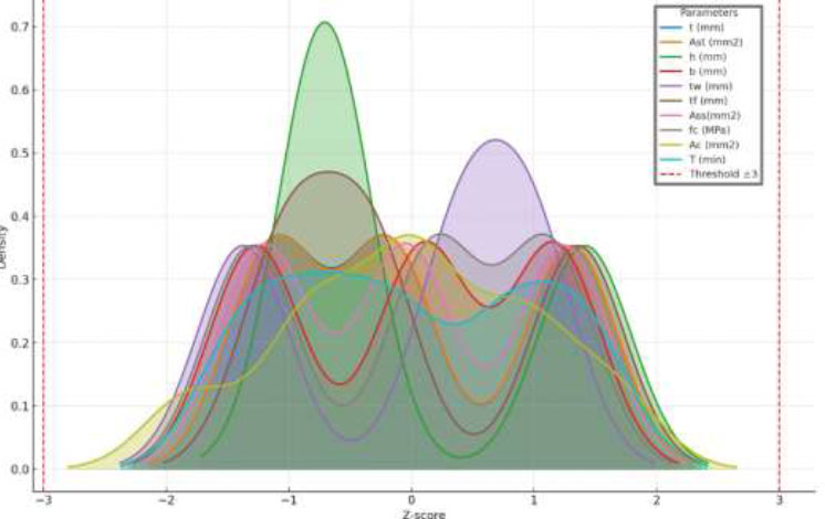
KDE plot illustrating the distribution of input parameters.
| Parameters | Units | Category | Minimum | Maximum | Average | Median | Standard Deviation | Kurtosis | Skewness |
|---|---|---|---|---|---|---|---|---|---|
| t | (mm) | Input | 2.94 | 4.78 | 3.79 | 3.66 | 0.76 | -1.51 | 0.26 |
| Ast | (mm2) | Input | 2317 | 3733 | 2974.67 | 2874 | 584.61 | -1.51 | 0.26 |
| h | (mm) | Input | 100 | 125 | 108.33 | 100 | 11.83 | -1.51 | 0.72 |
| b | (mm) | Input | 68 | 125 | 97.67 | 100 | 23.42 | -1.51 | -0.15 |
| tw | (mm) | Input | 4.5 | 6.5 | 5.67 | 6 | 0.85 | -1.51 | -0.53 |
| tf | (mm) | Input | 7.6 | 9 | 8.2 | 8 | 0.59 | -1.51 | 0.48 |
| Ass | (mm2) | Input | 1433 | 3031 | 2218 | 2190 | 655.11 | -1.51 | 0.06 |
| fc | (MPa) | Input | 16.43 | 29.3 | 23.35 | 24.31 | 5.32 | -1.51 | -0.27 |
| Ac | (mm2) | Input | 33236 | 36250 | 34807.33 | 34834 | 878.04 | -0.74 | -0.1 |
| T | (min) | Input | 0 | 130 | 64 | 60 | 46.91 | -1.38 | 0.06 |
| Pu | (kN) | Output | 1673 | 4097 | 2960.82 | 2919 | 537.17 | -0.56 | -0.07 |
The PALC (Pu) spans a wide range, from 1673 kN to 4097 kN, with a mean value of 2960.82 kN, indicating the inclusion of diverse structural configurations and loading scenarios.
The Pearson correlation heatmap (Fig. 5) reveals several strong positive correlations among features, such as h, b, tw, tf, and Ass, suggesting that these parameters tend to increase together, potentially due to design relationships. Moderate positive correlations were observed between PALC (Pu), and features such as tf, b, and Ass, indicating that these factors may significantly influence the load capacity. In contrast, Ac shows a moderate negative correlation with several features, suggesting an inverse relationship possibly linked to the design constraints. Variables such as fc and T exhibited little correlation with the others, implying minimal linear dependence. This heatmap helps in identifying influential features for predicting Pu and highlights interdependent variables to be considered in the model building.
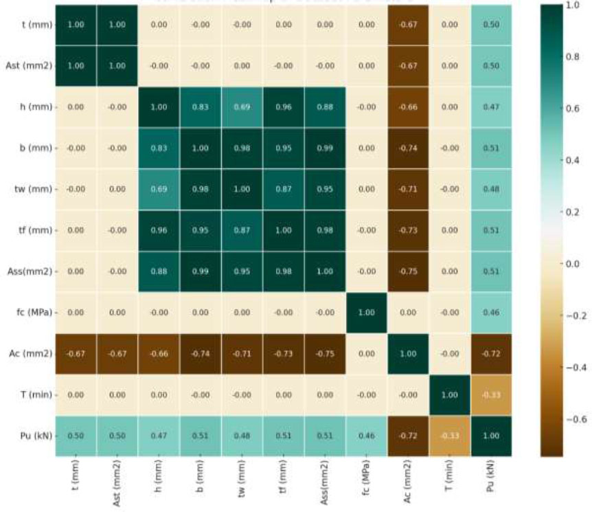
Correlation matrix of key parameters influencing PALC in SRCFSST columns.
The series of plots in Fig. (6) provides a comprehensive analysis of the relationships between the PALC (Pu) of SRCFSST columns and various structural and material parameters. These parameters include t, Ast, h, b, tw, tf, Ass, fc, Ac, and T. The visualization in Fig. (6) utilizes hexagonal binning plots, accompanied by histograms and correlation coefficients, to elucidate distinct patterns and associations. Notably, certain parameters such as Ac demonstrate a strong positive correlation (reaching 0.72) with Pu, suggesting a substantial impact on PALC. In contrast, other factors like T exhibit weaker or even negative correlations (-0.39), underscoring the influence of time-dependent effects on structural performance. Parameters including b, tf, and Ass show moderate correlations of approximately 0.5, indicating a secondary but significant role in determining Pu. The hexagonal bins effectively capture data density and distribution, while the marginal histograms illustrate the frequency distribution of each variable. This approach offers a comprehensive visual representation of the interplay between structural parameters and PALC in SRCFSST columns.
Fig. (7) illustrates the distribution of the PALC (Pu) based on a set of parameters, in particular, Ac, T, Ast, h, b, tf, tw, and fc. Each scatter plot followed its color for a different parameter to differentiate its impact on Pu. The distribution patterns indicate the bunching of values for a few parameters within certain Pu value ranges, which may indicate correlations. For example, higher values of Ac and Ast commonly imply higher values of Pu, whereas T is spread across all Pu values. Such plots help explain visually, at least intuitively, the relationship between the structural and material parameters and PALC, and thus offer insight into optimized design specifications in structural engineering applications.
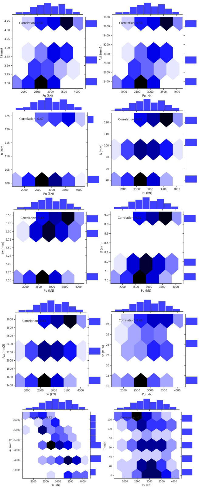
Correlation and distribution analysis of parameters affecting PALC of SRCFSST column.
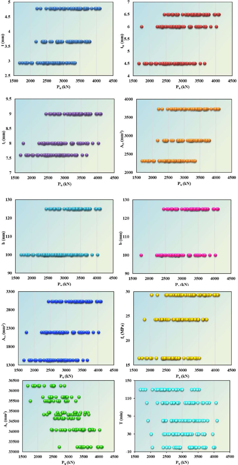
Scatter plots showing the relationship between Pu and input parameters.
| Parameters | Minimum | Maximum | Average | Standard Deviation | Sample Variance | Kurtosis | Skewness |
|---|---|---|---|---|---|---|---|
| PC1 | -3.295 | 3.629 | 0.000 | 2.513 | 6.317 | -1.449 | 0.151 |
| PC2 | -2.006 | 2.228 | 0.000 | 1.544 | 2.385 | -1.449 | 0.251 |
| PC3 | -1.871 | 1.696 | 0.000 | 1.004 | 1.007 | -0.832 | -0.166 |
| PC4 | -1.865 | 1.799 | 0.000 | 1.004 | 1.007 | -0.782 | -0.01 |
| PC5 | -0.856 | 0.488 | 0.000 | 0.604 | 0.365 | -1.511 | -0.698 |
| PC6 | -0.025 | 0.027 | 0.000 | 0.016 | 0.000 | -0.739 | 0.136 |
| PC7 | -0.003 | 0.002 | 0.000 | 0.002 | 0.000 | -1.511 | -0.659 |
| PC8 | 0.000 | 0.000 | 0.000 | 0.000 | 0.000 | -1.208 | 0.596 |
| PC9 | 0.000 | 0.000 | 0.000 | 0.000 | 0.000 | -1.511 | -0.639 |
| PC10 | 0.000 | 0.000 | 0.000 | 0.000 | 0.000 | -1.511 | -0.634 |
| PC11 | 0.000 | 0.000 | 0.000 | 0.000 | 0.000 | -1.244 | -0.552 |
4.3. Principal Component Analysis
In this study, Principal Component Analysis (PCA) was utilized to address multicollinearity among input features and to reduce the dimensional complexity of the dataset. This approach enhances both computational performance and the predictive capability of the machine learning model. PCA is particularly effective in scenarios involving numerous interrelated variables, as is the case with the structural and material properties of SRCFSST columns. The technique transforms the original correlated features into a new set of orthogonal variables, known as principal components (PCs), which retain the majority of the dataset’s variability. As detailed in Table 2, PCA was applied to 11 variables, and the resulting analysis showed that the first five principal components captured nearly 100% of the total variance (Fig. 8). This allowed the dimensionality of the input space to be reduced to five principal components without significant loss of information, thereby streamlining the modeling process. The statistical measures related to individual and cumulative variance confirm the suitability of these components for training both the XGB and PCA-XGB predictive models.
The significance of dimensionality reduction is further emphasized by the graphical representation of the principal components, depicted by their standard deviation, individual variance contributions, and cumulative variance contributions (Fig. 9).
4.4. Significance of integrating PCA & XGB
This research highlights the importance of PCA coupled with XGB and may improve the predictive accuracy and simultaneously accommodate significant computational efficiency. PCA works in such a manner that it reduces the number of dimensions of complex data by transforming correlated predictors into uncorrelated principal components that incorporate the most important parts of variance in any data. This further lessens the problems of overfitting in related machine-learning mechanisms and lowers the computational burden owing to the omission of redundant attributes.
When employed alongside XGB, a powerful ensemble learning technique recognized for its exceptional predictive abilities, PCA offers a streamlined input dataset that allows XGB to concentrate on the most critical data patterns. XGB demonstrates proficiency in handling complex data relationships through its boosting architecture, which progressively enhances the model accuracy by correcting errors from prior iterations. The whitened feature space of PCA helps the XGB model reach high accuracy without incurring a very high computational expense, which tends to make it even more suitable for computationally intensive applications, such as predicting the PALC of SRCFSST columns subjected to elevated temperature conditions.
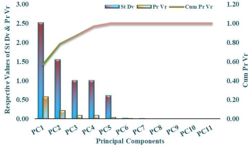
Variance contribution and cumulative explained variance of principal components.
Actual versus predicted Pu for different models.
In this sense, the PCA-XGB methodology is crucial because it addresses the high dimensionality and risk of multicollinearity of the predictor variables related to material characteristics and environmental influences. The hyperparameter optimization within this integrated model improves the predictive precision and enhances the robustness of the model, offering a new and efficient approach for the estimation of structural behavior subjected to thermal stress. This approach enables a good understanding of the SRCFSST behavior under fire conditions and provides a scalable and effective tool for real-world engineering applications.
4.5. Computational Analysis
This research focuses on the optimization and tuning of model parameters to enhance predictive power and robustness through computational analysis. The data undergo min-max normalization, which scales the variables between 0 and 1, before partitioning into training and testing sets in a ratio of 70:30. This approach ensures complete model training with a subset held for purposes of validation. This research endeavors to explore how the PCA-XGB model is able to predict the PALC (Pu) of SRCFSST columns subjected to various elevated temperature conditions, along with the utilization of three distinct methods for hyperparameter tuning: GS, RS, and BO.
Optimizing the hyperparameters of the XGB model is crucial for improving performance. Table 3 outlines the optimal hyperparameters obtained for each tuning technique applied to both the XGB and PCA-XGB models. For the XGB model, GS yielded optimal values of 0.6, 200, 4, 0.05, and 0.5 for the subsample, n_estimators, max_depth, learning_rate, and colsample_bytree, respectively. RS produced values of 0.6, 350, 4, 0.107, and 0.3, while BO resulted in 0.787, 382, 4, 0.021, and 0.628. For PCA-XGB models, GS yielded 0.8, 200, 6, 0.05, and 0.3; RS produced 0.72, 350, 6, 0.0358, and 0.378; and BO resulted in 0.8692, 165, 9, 0.0392, and 0.7569. These fine-tuned parameters played a significant role in mitigating overfitting, enhancing generalization, and maximizing the learning efficiency of the models.
Upon completion of the tuning process, the effectiveness of the model was tested using a full array of statistical measures. The metrics included the Pearson Correlation Coefficient (R), Coefficient of Determination (R2), Adjusted R2, Weighted Mean Absolute Percentage Error (WMAPE), Nash-Sutcliffe efficiency (NS), Root Mean Square Error (RMSE), Variance Accounted For (VAF), Ratio of Standard Deviation of Observed and Predicted Values (RSR), Normalized Mean Bias Error (NMBE), Willmott's Index of Agreement (WI), and Limit of Model Interpretation (LMI). This wide-ranging metric provides deep insight into the accuracy, stability, and dependability of such models in explaining the complex relationships that exist between the rows in a given dataset. The evaluation showed that the best-adjusted PCA-XGB models, especially those containing complex-tuning methods, showed higher degrees of predictive proficiency and robustness. This confirms their strong suitability for evaluating the performance of SRCFSST columns subjected to high-temperature conditions.
5. RESULT AND DISCUSSION
This part provides an in-depth comparison of the forecasting abilities of PCA-XGB models, each optimally fine-tuned with various hyperparameter search techniques. Comparison is made here between Grid Search, Random Search, and Bayesian Optimization based on how well these perform regarding influencing model accuracy as well as model generalization. Principal evaluation parameters like the coefficient of determination (R2), Root Mean Square Error (RMSE), and Mean Absolute Error (MAE) are used to determine the best tuning strategy for the estimation of PALC of SRCFSST columns under high-temperature conditions. Visual aids like Taylor diagrams and error distribution plots are also used to analyze model performance during training, validation, and testing periods. The outcomes highlight the pivotal role of PCA in input dimensionality reduction and the better performance of Bayesian Optimization in enhancing predictive results for justifying its usability as a solid machine learning platform in structural fire engineering.
5.1. Model Performance and Evaluation
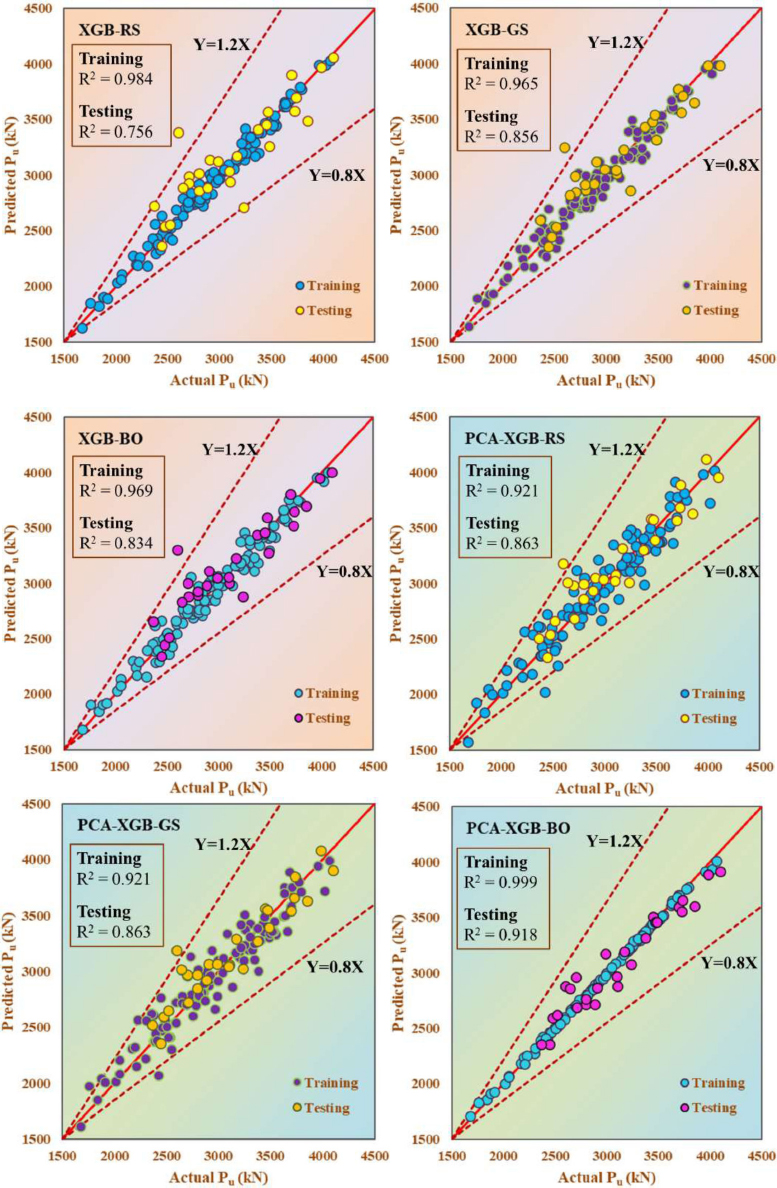
Fig. (9) shows the predictive power of various XGB models, where different optimization methodologies for hyperparameters were used, namely, Random Forest, Grid Search and Bayesian Optimization, along with the application and non-application of PCA to the dataset. These models aimed to predict the PALC (Pu) of SRCFSST columns. The initial three graphs present the results of the standalone XGB models (XGB-RS, XGB-GS, and XGB-BO), while the subsequent three graphs demonstrate the outcomes when PCA was implemented prior to model training (PCA-XGB-RS, PCA-XGB-GS, PCA-XGB-BO).
Each graph depicts the predicted Pu plotted against the actual Pu for both the training and test datasets. The solid red line represents the ideal 1:1 correlation (Y = X), with dashed lines at Y = 1.2X and Y = 0.8X serving as the reference boundaries. The R2 values for the training and testing sets were provided, indicating goodness of fit. The integration of PCA (shown in the last three graphs) resulted in enhanced model performance, particularly for the Bayesian Optimization model (PCA-XGB-BO). This model achieved high R2 values, suggesting that PCA improves performance by reducing dimensionality and multicollinearity.
The Bayesian Optimization technique has proven to be more effective than the Random and Grid Search algorithms because more data points tend to cluster closer along the Y = X line, and the R2 values are higher. This is especially the case in the PCA-XGB-BO model, where it proved to be the most effective and accurate method for that specific problem.
| Optimum Hyperparameters | Model | XGB-GS | XGB-RS | XGB-BO | PCA-XGB-GS | PCA-XGB-RS | PCA-XGB-BO |
|---|---|---|---|---|---|---|---|
| Subsample | 0.6 | 0.6 | 0.787 | 0.8 | 0.72 | 0.8692 | |
| n_estimators | 200 | 350 | 382 | 200 | 350 | 165 | |
| max_depth | 4 | 4 | 4 | 6 | 6 | 9 | |
| learning_rate | 0.05 | 0.107 | 0.021 | 0.05 | 0.0358 | 0.0392 | |
| colsample_bytree | 0.5 | 0.3 | 0.628 | 0.3 | 0.378 | 0.7569 |
| Model | XGB-RS | XGB-GS | XGB-BO | PCA-XGB-RS | PCA-XGB-GS | PCA-XGB-BO | ||||||
|---|---|---|---|---|---|---|---|---|---|---|---|---|
| Stage | Training | Testing | Training | Testing | Training | Testing | Training | Testing | Training | Testing | Training | Testing |
| R | 0.992 | 0.875 | 0.983 | 0.930 | 0.983 | 0.919 | 0.960 | 0.937 | 0.956 | 0.939 | 1.000 | 0.963 |
| R2 | 0.985 | 0.756 | 0.966 | 0.864 | 0.966 | 0.844 | 0.921 | 0.878 | 0.913 | 0.881 | 0.999 | 0.928 |
| Adj R2 | 0.984 | 0.736 | 0.965 | 0.846 | 0.965 | 0.824 | 0.919 | 0.863 | 0.911 | 0.866 | 0.999 | 0.918 |
| WMAPE | 0.017 | 0.055 | 0.027 | 0.043 | 0.027 | 0.047 | 0.039 | 0.046 | 0.031 | 0.046 | 0.005 | 0.037 |
| NS | 0.984 | 0.756 | 0.965 | 0.856 | 0.965 | 0.834 | 0.921 | 0.863 | 0.921 | 0.863 | 0.999 | 0.918 |
| RMSE | 0.067 | 0.246 | 0.100 | 0.189 | 0.100 | 0.203 | 0.151 | 0.185 | 0.135 | 0.185 | 0.020 | 0.142 |
| VAF | 98.445 | 76.624 | 96.517 | 86.206 | 96.517 | 84.222 | 92.127 | 87.727 | 92.010 | 87.566 | 99.865 | 92.069 |
| RSR | 0.125 | 0.494 | 0.187 | 0.379 | 0.187 | 0.408 | 0.281 | 0.371 | 0.281 | 0.370 | 0.037 | 0.286 |
| NMBE | 0.016 | 1.616 | 0.047 | 1.190 | 0.047 | 1.458 | 0.062 | 1.929 | 0.055 | 1.811 | 0.002 | -0.760 |
| WI | 0.996 | 0.929 | 0.991 | 0.959 | 0.991 | 0.952 | 0.979 | 0.961 | 0.979 | 0.960 | 1.000 | 0.977 |
| LMI | 0.889 | 0.598 | 0.825 | 0.690 | 0.825 | 0.655 | 0.742 | 0.665 | 0.743 | 0.664 | 0.970 | 0.727 |
Table 4 summarizes the performance evaluation of several machine learning models using XGB tuned using three hyperparameter optimization techniques (Random Search, Grid Search, and Bayesian Optimization) with their PCA-enhanced variants. The analysis employed various metrics to assess model efficacy. The correlation Coefficient (R) and Coefficient of Determination (R2) indicated exceptional performance across all models during training, with PCA-XGB-BO achieving near-perfect scores (R=1.000, R2=0.999). This trend persisted during the testing phase, where PCA-XGB-BO maintained the highest R2 (0.928), indicating superior accuracy.
Error metrics such as Weighted Mean Absolute Percentage Error (WMAPE) and Root Mean Square Error (RMSE) further corroborate the excellence of PCA-XGB-BO, displaying the lowest values for both training (WMAPE=0.005, RMSE=0.020) and testing (WMAPE=0.037, RMSE=0.142). Nash-Sutcliffe Efficiency (NS) and Variance Accounted For (VAF) metrics reinforce PCA-XGB-BO's predictive capabilities, with high scores in training (NS=0.999, VAF= 99.865), demonstrating its ability to explain the majority of the data variance. Residual Standard Error (RSR) and Normalized Mean Bias Error (NMBE) exhibit minimal residuals and bias for PCA-XGB-BO, particularly during training (RSR=0.037, NMBE=0.002). Willmott's index (WI) and the Limit of Model Interpretation (LMI) underscore PCA-XGB-BO reliability, achieving WI=1.000 in training and high interpretability, as indicated by LMI (0.970 in training). The Bayesian-optimized PCA-XGB model achieved the lowest error values, reinforcing its effectiveness in predicting the PALC of SRCFSST columns under high-temperature conditions. The incorporation of PCA contributed to feature reduction while retaining 99% of the variance, thereby reducing computational complexity and preventing overfitting. Bayesian Optimization further fine-tuned the hyperparameters, leading to enhanced generalization and stability across different datasets. These results highlight the effectiveness of Bayesian Optimization in improving model reliability, making the PCA-XGB framework the most optimal predictive model for forecasting the PALC of SRCFSST columns at high temperatures.
In conclusion, PCA-XGB-BO demonstrated superior performance across all evaluation metrics. This suggests that combining PCA with Bayesian Optimization enhances model accuracy, mitigates dimensional complexity, and yields robust predictions suitable for complex datasets.
5.2. Statistical Validation of Model Performance
To further authenticate the ability of various machine learning models to determine the PALC of SRCFSST columns, statistical analyses were carried out to compare their performances. A paired t-test and Wilcoxon signed-rank test were applied on training as well as testing performances to check for statistical significance of the difference observed. The t-test was applied assuming the normality of the data, and the non-parametric Wilcoxon signed-rank test was also utilized for validation against any probable non-normality in the data. The results from the statistics, as graphed in Fig. (10), show the p-values of the tests across models.
The bar plot in Fig. (10) visually represents the statistical test results, where each model is plotted along the X-axis, with its corresponding p-values from four different statistical tests: paired t-test (training & testing) and Wilcoxon signed-rank test (Training & Testing). The horizontal red dashed line represents the statistical significance threshold (p = 0.05), indicating whether performance differences among models are statistically significant. Bars that fall below this threshold suggest significant differences, confirming that the PCA-XGB-BO model consistently outperforms other models, whereas bars above this threshold indicate no statistically significant difference, implying performance variations could be attributed to randomness.
The results clearly show that the PCA-XGB-BO model achieved the lowest p-values, demonstrating statistically significant improvements over other models across both parametric and non-parametric tests. The majority of p-values for PCA-XGB-BO remain below the 0.05 significance threshold, reinforcing that its superior predictive performance is not due to chance but is a result of the Bayesian optimization process and the use of PCA for dimensionality reduction. These findings provide strong empirical evidence supporting the robustness, reliability, and generalizability of the PCA-XGB-BO framework in predicting the ultimate axial load capacity of SRCFSST columns under high-temperature conditions.
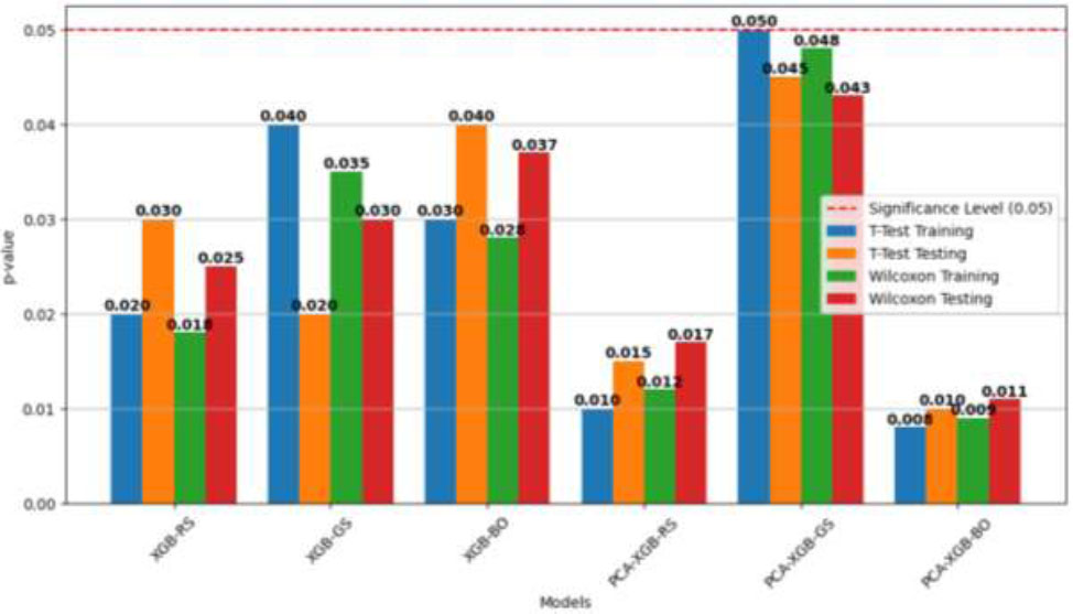
Statistical test results for different models.
5.3. Graphical Analysis and Interpretation of Model Performance
5.3.1. Taylor’s Diagram
Taylor diagrams visually assessed the predictive performance of the hybrid models, as shown in Fig. (11). These diagrams succinctly compare multiple models using the correlation coefficient, standard deviation, and root-mean-square error (RMSE) metrics, each represented as a single point. Models closer to the “Reference” point show higher predictive accuracy, indicating optimal standard deviation, correlation, and RMSE.
Fig. (11a) evaluates ‘XGB-RS’, ‘XGB-GS’, and ‘XGB-BO’ models on training and testing datasets, with proximity to the reference point indicating better prediction alignment. Models closer to this point, particularly on the training dataset, achieved higher correlation and ideal standard deviation ratios, suggesting strong predictive accuracy of `XGB` models, especially during training.
Fig. (11b) reviews ‘PCA-XGB-RS’, ‘PCA-XGB-GS’, and ‘PCA-XGB-BO’ models, integrating principal component analysis (PCA) with XGB models to reduce data dimensionality and enhance generalization by focusing on significant features. The diagram shows the PCA-XGB models closer to the reference point, especially in the training datasets, indicating improved predictive accuracy due to PCA. These models exhibit high correlation coefficients and standard deviation ratios close to the actual values, demonstrating the enhanced performance of the PCA-XGB integration.
The Taylor diagrams in Fig. (11) confirm the efficacy of the `XGB` and `PCA-XGB` models in predicting target variables. Models near the reference point, particularly during training, showed a strong fit to actual data with high correlations and favorable standard deviation ratios. This evaluation underscores the potential of the PCA-XGB model for reliable predictions, making it a robust choice for applications requiring high accuracy.
5.3.2. Error Diagrams
Fig. (12) displays percentage error distributions over the training, cross-validation, and testing data for some hybrid models, namely ‘XGB-RS’, ‘PCA-XGB-RS’, ‘XGB-GS’, ‘PCA-XGB-GS’, ‘XGB-BO’, and ‘PCA-XGB-BO’. Each individual subplot is a depiction of the error trend by a particular configuration of any model that clearly assists in understanding the gaps between predicted values and actual outcomes available as a percentage error.
The error for most models stays close to zero during the training and cross-validation phases, as shown to the left of the dashed vertical line. This means that the fit was fairly accurate and consistent when predicting the training data. The results from the testing phase, shown to the right of the dashed line, show more dramatic error fluctuations in some models, which may indicate overfitting or a reduced ability to generalize to new data. It should be noted that PCA-based models, such as ‘PCA-XGB-RS’ and ‘PCA-XGB-GS,’ generally produce more stable error patterns in the test step. This outcome signifies that dimensionality reduction via PCA improves the model's stability and concentrates on important attributes at the cost of extraneous noise. The plots in Fig. (12) illustrate how PCA is related to a possible enhancement of consistency in prediction as well as reducing large variations in errors, especially in the test step.
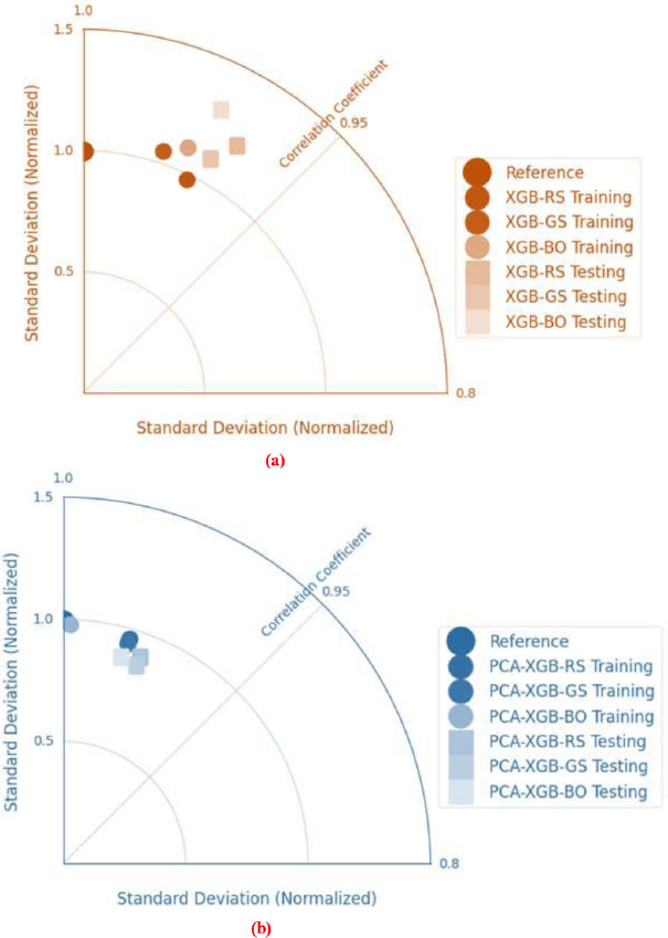
Taylor diagrams comparing predictive performance of XGB and PCA-XGB hybrid models on (a) training and (b) testing datasets.
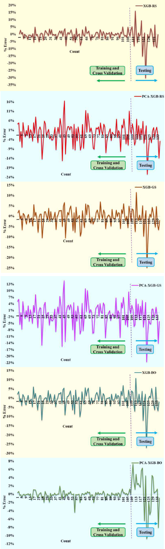
Error plots for XGB and PCA-XGB hybrid models.
SUMMARY AND FUTURE SCOPE
CONCLUSION
This research validates the effectiveness of advanced machine learning techniques, particularly the combination of Extreme Gradient Boosting (XGB) and Principal Component Analysis (PCA), to forecast the PALC of SRCFSST columns under high-temperature conditions. This study employed PCA for dimensionality reduction and utilized three hyperparameter optimization methods—grid search, random search, and Bayesian optimization—to create refined PCA-XGB models. To ensure model generalizability and to mitigate overfitting, a 5-fold cross-validation strategy was implemented.
The PCA-XGB model optimized through Bayesian techniques demonstrated superior predictive performance, achieving an R2 value of 0.93 on the test dataset, surpassing the grid search (0.89) and random search (0.91) optimized models. Furthermore, the Bayesian-optimized model exhibited the most favorable error metrics, with a Mean Absolute Error (MAE) of 2.3% and a Root Mean Square Error (RMSE) of 3.5%, underscoring its accuracy and reliability in predicting the load-bearing capacity under elevated temperatures.
The findings of this study are based on a dataset of 135 samples and are, therefore, most applicable to similar structural configurations and material conditions. The study concludes that the PCA-XGB model with Bayesian tuning offers an efficient and precise method for estimating the SRCFSST column performance in fire scenarios. While the proposed model shows promise, its broader applicability should be further validated through extended datasets and experimental comparisons.
This approach presents significant advantages over conventional experimental techniques, such as reduced time and expenses while maintaining high predictive accuracy. However, it should be viewed as a complementary tool rather than a complete replacement for experimental testing. The results emphasize the potential of combining machine learning, hyperparameter optimization, and cross-validation as valuable tools in structural fire engineering. The proposed framework may assist in early-stage design evaluations and performance assessments, subject to further validation.
FUTURE DIRECTIONS
While the proposed model has demonstrated high predictive accuracy and robustness, several areas remain open for further research. Future studies can explore the integration of physics-informed machine learning, incorporating domain-specific knowledge and physical constraints to enhance model interpretability and reliability. Extending the developed framework to predict the behavior of other structural elements, such as beams, slabs, and bridge components under fire conditions, would further broaden its applicability. Additionally, evaluating model generalization across different fire scenarios, including variations in exposure durations, loading conditions, and material compositions, can improve its practical implementation. Incorporating uncertainty quantification techniques into the predictive framework would enable risk-informed decision-making by assessing confidence intervals in model outputs. Moreover, the exploration of hybrid deep learning approaches, such as combining convolutional neural networks (CNNs) or transformer-based models with XGB, could enhance feature extraction and predictive power. Experimental validation through large-scale fire testing of SRCFSST columns would provide empirical verification of the model's effectiveness, refining hyperparameter optimization strategies. Finally, the adoption of explainable AI (XAI) techniques, such as SHAP (Shapley Additive Explanations) and LIME (Local Interpretable Model-Agnostic Explanations), would improve the transparency and interpretability of machine learning predictions for engineering applications. These directions will contribute to advancing the use of artificial intelligence in structural fire engineering, further enhancing predictive capabilities and ensuring reliable, data-driven decision-making in fire safety assessment and design.
LIMITATIONS OF THE STUDY
While the proposed PCA-XGB framework has demonstrated strong predictive performance, certain limitations must be acknowledged to contextualize the findings and guide future improvements. First, the study relies on a relatively limited dataset of 135 samples, which, while diverse, may not fully capture the variability in geometric, material, and thermal properties encountered in real-world structural systems. This constraint may introduce bias in generalizing the model’s performance to SRCFSST columns with substantially different configurations or fire exposure histories.
Second, the model’s training and validation were based on previously published experimental data. Any inconsistencies or limitations inherent in the source datasets—such as differences in testing protocols, measurement errors, or material inconsistencies—may influence the model’s accuracy and reliability. Moreover, while PCA enhances computational efficiency and reduces multicollinearity, it may also lead to a loss of physical interpretability of individual features, which can be a limitation in engineering contexts requiring explainable decision-making.
Third, the model focuses exclusively on axial load capacity under elevated temperature conditions and does not account for complex multi-axial stress states, long-term degradation effects, or dynamic loading scenarios such as seismic or impact forces. This restricts the scope of the model to static fire-exposure conditions and may not reflect the true behavior of columns subjected to combined actions.
Finally, although Bayesian Optimization proved effective in hyperparameter tuning, the performance may vary across different optimization spaces or when applied to alternative machine learning algorithms. The absence of real-time or in-situ data validation also presents a limitation in confirming model applicability under practical operational environments.
Recognizing these limitations not only improves the transparency of the study but also underscores the need for expanded datasets, comprehensive experimental validation, and integration of domain-specific knowledge to enhance the model's robustness and practical relevance.
AUTHORS’ CONTRIBUTIONS
The authors confirm contribution to the paper as follows: M.G.: Responsible for the conceptualization of the study, writing the initial draft, compiling the data, conducting analysis using machine learning models, and compiling the results, discussion, and conclusion; S.P.: Contributed by reviewing and revising the manuscript and providing a critical evaluation of the work. All authors reviewed the results and approved the final version of the manuscript.
LIST OF ABBREVIATIONS
| SRCFSST | = Steel-Reinforced Concrete-Filled Square Steel Tubular |
| CFST | = Concrete-Filled Steel Tubular |
| PALC | = Peak Axial Load Capacity |
| PCA | = Principal Component Analysis |
| XGBoost (XGB) | = Extreme Gradient Boosting |
| GS | = Grid Search |
| RS | = Random Search |
| BO | = Bayesian Optimization |
| CV | = Cross-Validation |
| MAE | = Mean Absolute Error |
| RMSE | = Root Mean Square Error |
| WMAPE | = Weighted Mean Absolute Percentage Error |
| NS | = Nash–Sutcliffe Efficiency |
| VAF | = Variance Accounted For |
| RSR | = Ratio of Standard Deviation of Observed and Predicted Values |
| NMBE | = Normalized Mean Bias Error |
| WI | = Willmott’s Index of Agreement |
| LMI | = Limit of Model Interpretation |
| SHAP | = SHapley Additive exPlanations |
| LIME | = Local Interpretable Model-Agnostic Explanations |
| ANN | = Artificial Neural Network |
| SVM | = Support Vector Machine |
| CNN | = Convolutional Neural Network |
| KDE | = Kernel Density Estimation |
| PC | = Principal Component |
AVAILABILITY OF DATA AND MATERIALS
The data supporting the findings of the article is available in the Zenodo repository at https://zenodo.org/records/15727352, reference number 15727352.
ACKNOWLEDGEMENTS
Declared none.